Linear versus Exponential Growth and Decay

Calculus 1, Lectures 3A and 3B

*For $f(x)=2\cdot 1.5^{x}$ , $f(x+2)=1.5^{2}f(x)$ , no matter what $x$ is.* The exponential function is converting addition of inputs to multiplication of outputs.

*For $f(x)=2\cdot 1.5^{x}$ , $f(x+2)=1.5^{2}f(x)$ , no matter what $x$ is.* The exponential function is converting addition of inputs to multiplication of outputs.

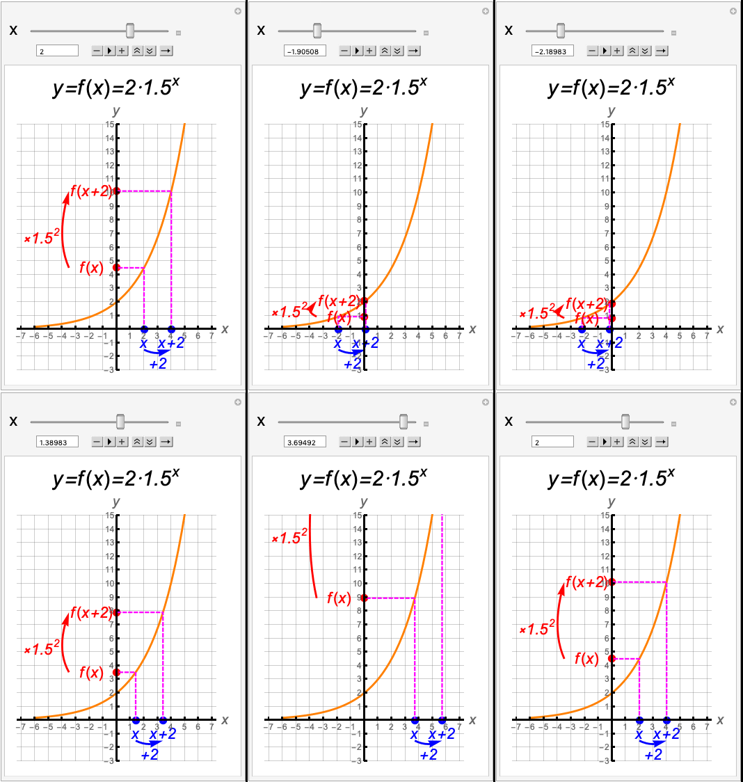
Linear functions are constructed from the arithmetic building blocks of repeated addition and subtraction. In a similar manner, exponential functions are constructed from repeated multiplication and division.

These sentences describe both the most basic similarity and the most basic contrast when comparing linear vs exponential functions.

Certainly the formulas for linear vs exponential functions are different. A linear function has the form $f(x)=mx+b$ , while an exponential function has the form $f(x)=a\cdot b^{x}$ .

But what does this mean about their behaviors? And how are these behaviors related to the first two sentences of this post?

Rates Which are Constant for Linear vs Exponential

In the post “Proportionality and Linear Functions”, I emphasized that linear functions that arise from proportional quantities have constant rates of change (slopes). This is true for linear functions in general, as is verified by the following calculation for $f(x)=mx+b$ .

$\frac{\Delta y}{\Delta t}=\frac{f(x+\Delta x)-f(x)}{\Delta x}=\frac{(m(x+\Delta x)+b)-(mx+b)}{\Delta x}=\frac{m\Delta x}{\Delta x}=m\mbox{ for }\Delta x\not=0.$

But why does this mean that linear functions are constructed from repeated addition and subtraction? We will explore the answer to that question further below.

On the other hand, exponential functions have constant relative (percent) rates of change over any given interval of constant length. This fact is verified by the calculation below for $f(x)=a\cdot b^{x}$ . You should realize that the expression $\frac{f(x+\Delta x)-f(x)}{f(x)}$ represents the relative (percent) rate of change for any function over an interval $[x,x+\Delta x]$ .

$\frac{f(x+\Delta x)-f(x)}{f(x)}=\frac{a\cdot b^{x+\Delta x}-a\cdot b^{x}}{a\cdot b^{x}}=\frac{a\cdot b^{x}(b^{\Delta x}-1)}{a\cdot b^{x}}=b^{\Delta x}-1.$

Note that the final quantity $b^{\Delta x}-1$ is independent of $x$ . This is why the relative (percent) rate of change of the function $f(x)=a\cdot b^{x}$ over any interval of length $\Delta x$ is constant.

But why does this mean that exponential functions are constructed from repeated multiplication and division? We explore this fact, along with the related fact for linear functions, in the section below.

Lecture 3A: Constructing Linear vs Exponential via Repeated Operations

About 20 minutes into Lecture 3A of my calculus series, I explore the differences between linear functions and exponential functions. This is done with two examples. One example is based on repeated addition and the other example is based on repeated multiplication.

Calculus 1, Lec 3A: Linear Equation Problem Solving, Exponential Function Growth & Decay Properties

In the video, the linear function is called $L(x)$ and the exponential function is called $E(x)$ . For both examples, the first value of $x$ considered is $x=3$ . In addition, both functions have the same value there: $L(3)=E(3)=6$ .

Constructing the Functions

Using $\Delta x=2$ , the values of $L(x)$ and $E(x)$ at $x=5,7,$ and $9$ are then “constructed”.

For $L(x)$ , I use repeated addition of 5 to get $L(5)=L(3)+5=6+5=11$ , $L(7)=L(5)+5=11+5=16$ , and $L(9)=L(7)+5=16+5=21$ .

On the other hand, for $E(x)$ , I use repeated multiplication of 5 to get $E(5)=5\cdot E(3)=5\cdot 6=30$ , $E(7)=5\cdot E(5)=5\cdot 30=150$ , and $E(9)=5\cdot E(7)=5\cdot 150=750$ .

Certainly then, $L$ has a constant rate of change (slope) of $\frac{5}{2}$ . Using the point-slope form of the equation of a line, we can also see that $L(x)=\frac{5}{2}(x-3)+6=\frac{5}{2}x-\frac{15}{2}+\frac{12}{2}=\frac{5}{2}x-\frac{3}{2}$ .

The function $E$ has a constant relative (percent) rate of change. Based on its values, this can be described as a $\frac{30-6}{6}=\frac{24}{6}=4=400\%$ increase in the output of $E$ for every 2 unit increase in $x$ . If you want to check this against the other values of $E$ , you’ll get $\frac{150-30}{30}=\frac{120}{3}=4=400\%$ and $\frac{750-150}{150}=\frac{500}{150}=4=400\%$ as well.

The multiplier 5 represents the value of $b^{2}$ for $E(x)=a\cdot b^{x}$ (note that $5-1=4=400\%$ as well). Therefore, $b=\sqrt{5}\approx 2.236$ , which represents $2.236-1=1.236=123.6\%$ growth in the value of $E(x)$ for each 1 unit increase of $x$ .

The formula for $E$ can be found to be $E(x)=6\cdot (\sqrt{5})^{x-3}=\frac{6}{5\sqrt{5}}(\sqrt{5})^{x}\approx 0.536656\cdot 2.236068^{x}$ .

Lecture 3B: More Details about Exponential Functions

One of the main points of emphasis in Lecture 3B is that it is useful to write exponential functions in various ways.

Calculus 1, Lecture 3B: Exponential Functions Fundamental Properties (also see the end of Lec 3A)

To quickly summarize the main idea, let $b>1$ so that $f(t)=a\cdot b^{t}$ is an exponential growth function. Then we can also write this function as $f(t)=a\cdot (1+r)^{t}=ae^{kt}=a\cdot 2^{t/T_{2}}$ , where $b=1+r=e^{k}\approx 2.71828182846^{k}$ and $T_{2}$ is the function’s doubling-time.

Exponential Growth Example

Let’s consider a particular example. Suppose you find an awesome bank account that gives you a guaranteed 10% annual rate of return. Assume interest is earned continuously (at every moment of every day).

Then, if you make a monetary deposit of 1000 at $t=0$ , your balance at time $t$ years is $f(t)=1000\cdot 1.1^{t}$ .

Therefore, the growth factor is $b=1.1$ , meaning that your ending amount each year is 110% of what you started with. On the other hand, the growth rate is $r=b-1=0.1=10\%$ , meaning your money grows by 10% each year.

We can contrast this with the value of $k$ . This value is $k=\ln(b)=\ln(1+r)=\ln(1.1)\approx 0.0953101798$ and we can write $f(t)\approx 1000\cdot e^{0.0953101798t}$ . The value $k\approx 0.0953=9.53\%$ represents the so-called continuous annual rate of growth.

Finally, the balance will double to 2000 when $f(t)=2000\Rightarrow 1000e^{0.0953101798t}=2000\Rightarrow t=\frac{\ln(2)}{0.0953101798}\approx 7.27$ years. This is the doubling time $T_{2}\approx 7.2725409$ years. We can therefore write $f(t)\approx 1000\cdot 2^{t/7.27}$ .

Exponential Decay Example

For exponential decay, the factor $b$ satisfies $0<b<1$ . In other words, it represents decay.

This means $r=b-1<0$ and $k=\ln(b)=\ln(1+r)<0$ . It also means that there is a half-life to focus on, rather than a doubling-time.

One of the main applications of exponential decay is to radioactive decay. However, we can also consider an application to auto depreciation. If a car is initially bought for $20000 and the value decays at a rate of 15% per year, how does its value $f(t)$ depend on time?

With a bit of thought, we quickly see that the answer is $f(t)=20000\cdot 0.85^{t}$ , since 0.85 is 15% less than 1. Therefore $b=0.85$ is now the annual decay factor.

From this, we get $r=b-1=-0.15=-15%$ as the growth rate (which represents decay rate $|r|=15\%$ ). We also get $k=\ln(b)=\ln(1+r)=\ln(0.85)\approx -0.1625189=-16.25189\%$ as the continuous growth rate (which represents continuous decay rate $|k|=16.25189\%$ ).

Finally, for the half-life, the time to decay to half the value, do the following calculation:

$10000=20000\cdot e^{-0.1625189t}\Rightarrow t=-\frac{\ln(2)}{-0.1625189}\approx 4.265025\mbox{ years}.$

Hence, $f(t)\approx 20000\cdot \left(\frac{1}{2}\right)^{t/4.265025}=20000\cdot 2^{-t/4.265025}$ .

This is the most natural way to represent the function if you are imagining that a certain number of half-lives have elapsed. For example, if 2 half lives have elapsed (which represents about $8.53$ years), then $f(t)=20000\cdot 2^{-2}=5000$ .