Financial Mathematics Tools: Substitutions, Quadratic Formula, Logarithms, and "Functional-Thinking"

Useful pre-university mathematics is not restricted to arithmetic, percentages, and basic algebra.

Functional-thinking is one key to doing many other useful things. Tools such as substitutions, the quadratic formula, and logarithms also come in handy.

These tools are used in engineering and science. For example, in the evaluation of useful integrals (such as those that come up in Fourier analysis applied to signal processing), the analysis of the motion of a projectile, and the determination of the half-life of a radioactive substance. But these tools can be useful in financial mathematics as well.

It is also the case that what I call “functional-thinking” is very powerful, including in financial mathematics. What do I mean by this? I mean that, as much as possible, your mathematical thinking should be dominated by the desire to conceptualize equations as defining functions that can often be graphed and analyzed, sometimes using calculus to help. This is especially fruitful when you have a computer-algebra system (CAS) such as Wolfram Research‘s Mathematica. It can do a lot of the calculations and graphing for you; freeing you up to ask questions, make conjectures, and draw interesting and useful conclusions.

Solving for Two Unknown Equally Spaced Deposit Times: The Power of Functional-Thinking

In the video below, I solve a financial mathematics problem. A person named Tina makes two deposits that are equally spaced in time after time $t=0$ . Therefore, we can say that they occur at times $n$ and $2n$ . Another person, named Joe, has an account that grows using simple interest. We assume that Tina’s account grows using compound interest to the same final accumulated amount (future value) as Joe’s at time $t=T$ (where $T=10$ in the video). The goal is then to solve for $n$ .

Generalizing the Problem

Tina has two specific deposit amounts at a specific interest rate in the video. However, I want to emphasize the importance of generalizing to my audience for this blog. So I will use general symbols (letters) for these quantities. Generalizing and handling symbolic equations with many arbitrary quantities are important skills for improving your mathematical abilities. These things will also help us emphasize the importance of functional-thinking near the end of this post.

So suppose that Tina deposits amount $A$ at time $n$ and amount $B$ at time $2n$ . Suppose further that the accumulated value at time $t=T$ is $C$ . The timeline for this situation is shown in the picture below.

Financial timeline for the generalized problem — Deposits of $A$ and $B$ occur at times $n$ and $2n$ , respectively. Their combined accumulated (future) value at time $T$ is $C.$

Deposits of $A$ and $B$ occur at times $n$ and $2n$ , respectively. Their combined accumulated (future) value at time $T$ is $C.$

It should be pointed out that neither $n$ nor $T$ is required be an integer here; though in real life, compound interest is often only paid at integer or discrete rational values of time. Because of this complicating factor, whatever answers we get should be considered to be approximations in many situations.

Deposit $A$ is compounding for time $T-n$ while deposit $B$ is compounding for time $T-2n$ . If the effective periodic interest rate is $i$ , then the combined future value is $A(1+i)^{T-n}+B(1+i)^{T-2n}$ . Therefore the equation of value is $A(1+i)^{T-n}+B(1+i)^{T-2n}=C$ .

Important side note: the interest rate in a problem may not always be given as an effective periodic rate, but rather a “nominal” rate that is compounded a certain number of times per period.

Using Logarithms

There are six arbitrary quantities $A, B, C, i, T,$ and $n$ , but only $n$ is unknown. The fact that $n$ is in two exponents is the clue that a logarithm might be helpful. The fact that one of the exponents involves $n$ and another involves $2n$ is a more subtle hint that the quadratic formula might also be useful.

This is the point of the problem-solving process where both experience and symbolic-manipulation skills, using abstract properties of algebra (including exponent properties), is essential. Even with such skills, it may not always be clear whether your manipulations will produce something useful. Keep at it! Don’t be afraid to do some scratch work along the side of your paper.

Rewriting the Equation of Value in a Form Leading to the Use of a Substitution and the Quadratic Formula

As mentioned above, the equation of value is $A(1+i)^{T-n}+B(1+i)^{T-2n}=C,$ and our goal is to solve for $n$ . First, by laws of exponents, this may be rewritten as $A(1+i)^{T}(1+i)^{-n}+B(1+i)^{T}(1+i)^{-2n}=C.$

This form of the equation has the benefit of highlighting a common factor on the left-hand side, $(1+i)^{T}$ . We next factor this out to get $(1+i)^{T}(A(1+i)^{-n}+B(1+i)^{-2n})=C$ .

Now divide both sides of this equation by the nonzero quantity $(1+i)^{T}$ . This gives $A(1+i)^{-n}+B(1+i)^{-2n}=\frac{C}{(1+i)^{T}}$ . Next, rearrange by subtraction to get $B(1+i)^{-2n}+A(1+i)^{-n}-\frac{C}{(1+i)^{T}}=0$ .

Now we start to get an inkling that the quadratic formula might be helpful. Indeed, by another law of exponents, we know that $(1+i)^{-2n}=((1+i)^{-n})^{2}$ , so our equation is $B((1+i)^{-n})^{2}+A(1+i)^{-n}-\frac{C}{(1+i)^{T}}=0.$

This is the point where a mathematical substitution is helpful. What is a mathematical substitution? It’s really just a way of rewriting an equation so it looks simpler. How? By making a replacement. In the present situation, replace $(1+i)^{-n}$ with some simpler symbol, like another letter; say $u=(1+i)^{-n}$ . Since the constant term is somewhat complicated, we might also want to use a substitution for that; say $v=-\frac{C}{(1+i)^{T}}=-C(1+i)^{-T}$ . After making these definitions, the equation of value becomes $Bu^{2}+Au+v=0.$

This is a quadratic equation in the unknown quantity $u$ , with zero on one side. Hence, the quadratic formula can be used to solve for $u$ , giving

$u=\frac{-A\pm \sqrt{A^{2}-4Bv}}{2B}=\frac{-A\pm \sqrt{A^{2}+4BC(1+i)^{-T}}}{2B}.$

Using a Logarithm to Finish

Since $u=(1+i)^{-n}$ , use a logarithm to find $n$ as a function of $u$ and $i$ . In most situations where calculus might be handy, use the natural logarithm (log base $e$ ), $\ln(x)$ . Applying this function to both sides of $u=(1+i)^{-n}$ and using properties of logarithms gives $\ln(u)=\ln((1+i)^{-n})=-n\ln(1+i)$ . Therefore, $n=-\frac{\ln(u)}{\ln(1+i)}.$

Now replace $u$ with the expression two paragraphs above. Then take the positive square root (since $u>0$ ) to get our somewhat wild-looking final answer:

$n=-\frac{1}{\ln(1+i)}\ln\left(\frac{-A+ \sqrt{A^{2}+4BC(1+i)^{-T}}}{2B}\right)$

The Power of Functional-Thinking

Was all this generality worth it? I think so. Let me try to convince you.

First, take the equation above and think of it as defining $n$ as a function of the other quantities. Using notation from multivariable calculus, we could write, for instance:

$n=f(A,B,C,i,T)=-\frac{1}{\ln(1+i)}\ln\left(\frac{-A+ \sqrt{A^{2}+4BC(1+i)^{-T}}}{2B}\right)$

In other words, $n=f(A,B,C,i,T)$ defines a function $f$ of five independent variables and one dependent variable $n.$

Remind yourself what this represents. For a given first deposit $A$ , second deposit $B$ , future time $T$ , effective periodic interest rate $i$ , and accumulated value $C$ at time $T$ , the output of this function gives the value $n$ at which the first deposit is made and the value $2n$ at which the second deposit is made.

For the example from the video above, you can use your calculator to check that $f(10,30,67.5,0.0915,10)\approx 2.325$ . This is the final answer, in years, derived in the video.

Solving Infinitely Many Problems at Once with Functional Thinking

This function now helps us to solve infinitely many other problems of the same type. All without having to re-do our work! Hey!…Infinity is Really Big! Suppose, for example, that the deposit at time $n$ is $A=20$ , the deposit at time $2n$ is $B=40$ , the future value is $C=100$ , the effective annual interest rate is $i=0.052$ , and the future time is $T=25$ . You should check with your calculator that the first deposit occurs at time $n=f(20,40,100,0.052,25)\approx 9.257$ years.

Even more impressively and importantly, however, graphs of this function can help us understand it more deeply and conceive of other relevant questions to ask and answer.

How can this be? How can we make the graph of such a higher-dimensional function? Isn’t that impossible?

If you thought of these questions, that’s not surprising. No human that I know of can accurately and “truly” visualize beyond three spatial-dimensions. However, a standard trick-of-the-trade in this situation is to look at “slices” of the “true” higher-dimensional graph.

Graphical Analysis

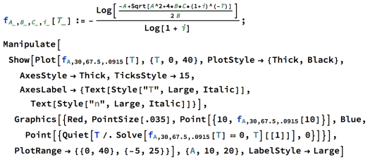
Since there are five independent variables and one dependent variable, the true higher-dimensional graph would be a five-dimensional “hypersurface” or “manifold” sitting inside $5+1=6$ -dimensional space. However, we can reduce this down to something we can visualize by setting most of the variables equal to constants.

For example, the figure below shows the graph of $n=g(T)=f(10,30,67.5,0.0915,T)$ as an “ordinary” graph of one independent variable $T$ . The red dot highlighted on the graph has coordinates $(T,N)=(10,g(10))=(10,f(10,30,67.5,0.0915,10))\approx (10,2.325)$ . Again, this represents the answer from the problem in the video. Technically-speaking, this graph is created by slicing the five-dimensional graph with a two-dimensional plane in six-dimensional space. Yeah…just try visualizing that as you go to sleep tonight…

A functional thinking illustration. This represents how the answer for the first deposit time depends on the final time for the future value. — The graph of $n$ as a function of $T$ when $A=10$ , $B=30$ , $C=67.5$ , and $i=0.0915$ . The coordinates of the red dot reflect the value of $n\approx 2.325$ when $T=10$ from the video. The blue dot has a second coordinate of zero, and first coordinate $T\approx 5.976$ , effectively telling us that when $T\leq 5.976$ , the problem cannot be solved for an answer that makes financial sense.

The graph of $n$ as a function of $T$ when $A=10$ , $B=30$ , $C=67.5$ , and $i=0.0915$ . The coordinates of the red dot reflect the value of $n\approx 2.325$ when $T=10$ from the video. The blue dot has a second coordinate of zero, and first coordinate $T\approx 5.976$ , effectively telling us that when $T\leq 5.976$ , the problem cannot be solved for an answer that makes financial sense.

But what does the blue dot represent? Notice that this graph has a horizontal T-intercept, where $n=0$ . The blue dot has a second coordinate $n=0$ . Its first coordinate can be approximated to be $T\approx 5.976$ . This can be interpreted as saying the following. When $A=10$ , $B=30$ , $C=67.5$ , and $i=0.0915=9.15\%$ , the original problem has no financially-meaningful solution when $T\leq 5.976$ (approximately). This is something we never may have even thought about without using functional-thinking and graphing.

Using Calculus and a Computer Algebra System (CAS)

This is again complicated enough that a CAS is extremely helpful. When I used Mathematica, here’s what I got for the simplified second derivative (with respect to $T$ , when $A=10, B=30, C=67.5,$ and $i=0.0915$ ).

$\frac{dn}{dT}=g'(T)\approx \frac{1772.95}{(8100+100\cdot 1.0915^{T})\sqrt{100+8100\cdot 1.0915^{-T}}}.$

This quantity is clearly always positive. Here’s what its graph looks like. Notice that it always is fairly small in value. It also does appear to approach zero at $T$ increases.

The second derivative helps us determine the concavity of the original graph in our functional-thinking generalization. — The second derivative of $n$ as a function of $T$ for the same given values of the other parameters as above. It is always positive and seems to decrease to zero as $T$ increases. So the graph of $n$ as a function of $T$ is always concave up, but indeed does “straighten out” while never becoming concave down as $T$ increases.

The second derivative of $n$ as a function of $T$ for the same given values of the other parameters as above. It is always positive and seems to decrease to zero as $T$ increases. So the graph of $n$ as a function of $T$ is always concave up, but indeed does “straighten out” while never becoming concave down as $T$ increases.

Other Graphs

Should we do anything else? How about graphing a function of two-variables? Let’s graph $n=h(A,T)=f(A,30, 67.5,0.0915,T)$ . This graph is formed by slicing the five-dimensional graph with a three-dimensional hypersurface in six-dimensional space, resulting in a two-dimensional surface in three-dimensional space (wow!). Here’s what it looks like. The figure is described by its caption.

Here we use functional thinking to see how the answer depends on two unknowns. — The graph of the time of initial deposit $n$ as a function of the initial deposit amount $A$ and the time for the future value evaluation $T$ . The red curve shows the slice of this curve where $T=10$ . The blue curve shows the slice of this curve where $n=0$ .

The graph of the time of initial deposit $n$ as a function of the initial deposit amount $A$ and the time for the future value evaluation $T$ . The red curve shows the slice of this curve where $T=10$ . The blue curve shows the slice of this curve where $n=0$ .

Finally, we can make a movie of slices of this surface. For example, we can show the graph of $n$ as a function of $T$ as $A$ increases. In such a movie we are slicing this surface with planes parallel to the $Tn$ -plane and moving it to the right as $A$ increases.

Animated graph of the answer as a parameter changes. This is like looking at slices of the previous graph in three dimensions. — Animation of the graph of $n$ as a function of $T$ as $A$ varies.

Animation of the graph of $n$ as a function of $T$ as $A$ varies.

One practical thing we see from this is that as $A$ increases, the $T$ -intercept of this graph decreases, meaning that the set of times $T$ for which the problem can be solved expands to include more and more low values of $T$ . Cool! Functional-thinking is really powerful!

Below is the Mathematica code for the animation above for those who are interested.

Mathematica code for our functional thinking animation.

Financial Mathematics Tools: Substitutions, Quadratic Formula, Logarithms, and “Functional-Thinking”