Transformed Power Function Survival Models

Studying for Exam LTAM, Part 1.10

A family of transformed power function survival functions $S_{0}(t)=1-\frac{t^{p}}{\omega^{p}}$ .

A family of transformed power function survival functions $S_{0}(t)=1-\frac{t^{p}}{\omega^{p}}$ .

A power function is defined by a formula of the form $f(t)=at^{p}$ for some constants $a$ and $p$ .

For certain choices of $a$ and $p$ , such a function could serve as the force of mortality for a continuous survival random variable $T_{0}$ . But it could not serve as a survival function for $T_{0}$ . This is because a survival function $S_{0}(t)$ must satisfy the conditions $S_{0}(0)=1$ and $\displaystyle\lim_{t\rightarrow \infty}S_{0}(t)=0$ .

However, if we transform a power function in certain ways, it can serve as a survival function. Two natural ways this can be done are shown below.

(Horizontally Reflected & Shifted Power Function — labeled $H$ ) $S_{0}(t)=\,_{t}p_{0}=\left(1-\frac{t}{\omega}\right)^{p}$ for $0\leq t\leq \omega$ and $p>0$ , and
(Vertically Reflected & Shifted Power Function — labeled $V$ ) $S_{0}(t)=\,_{t}p_{0}=1-\left(\frac{t}{\omega}\right)^{p}$ for $0\leq t\leq \omega$ and $p>0$ .

Note that $S_{0}(\omega)=0$ for both of these situations. It is also understood in both cases that $S_{0}(t)=0$ for $t>\omega$ . We omit reference to these values of $t$ in the rest of this article.

For ease of reference, these models will be labeled with the letters “H” and “V” as indicated above.

The Models as Transformed Power Functions

Model $H$ can be obtained from the power function $\frac{1}{\omega^{p}}t^{p}$ as follows. First, replace $t$ with $-t$ , which represents a horizontal reflection across the vertical axis. Next, replace $t$ with $t-\omega$ to get $-(t-\omega)=\omega-t$ , which represents a horizontal shift the right by $\omega>0$ units. The resulting function $S_{0}(t)=\,_{t}p_{0}=\frac{(\omega-t)^{p}}{\omega^{p}}=\left(\frac{\omega-t}{\omega}\right)^{p}$ is the same as the original for Model $H$ : $S_{0}(t)=\,_{t}p_{0}=\left(1-\frac{t}{\omega}\right)^{p}$ .

An animation showing these two transformations when $\omega=100$ and $p=2$ is shown below. The animation parameter is $\lambda$ . As $\lambda$ increases from 0 to 1, the original power function graph gets reflected across the vertical axis. Then, as $\lambda$ increases from 1 to 2, the reflected graph gets translated to the right.

Two-step transformation of a power function into Model $H$ when $\omega=100$ and $p=2$ .

A static graph of $S_{0}(t)=\,_{t}p_{0}=\left(1-\frac{t}{\omega}\right)^{p}$ when $\omega=100$ and $p=2$ is shown in the figure below. Since $p=2$ , this particular graph is a piece of a parabola.

Model $H$ survival function $S_{0}(t)=\,_{t}p_{0}=\left(1-\frac{t}{100}\right)^{2}$ for $0\leq t\leq 100$ . Note that this formula can also be written as *$S_{0}(t)=\,_{t}p_{0}=1-\frac{t}{50}+\frac{t^{2}}{10000}$ . It is more informative to keep it in the original form, however.*

Model $V$ is obtained from the power function $\frac{1}{\omega^{p}}t^{p}$ as follows. First, put a negative sign in front of this expression to get $-\frac{t^{p}}{\omega^{p}}$ , which represents a vertical reflection across the horizontal axis. Then add one to this expression, which represents a vertical shift upward by one unit, to get Model $V$ : $S_{0}(t)=\,_{t}p_{0}=1-\left(\frac{t}{\omega}\right)^{p}$ .

*Two-step transformation of a power function into Model $V$ when $\omega=100$ and $p=2$ .*

A static graph of $S_{0}(t)=\,_{t}p_{0}=1-\left(\frac{t}{\omega}\right)^{p}$ when $\omega=100$ and $p=2$ is shown in the figure below. Since $p=2$ , this particular graph is also a piece of a parabola.

*Model $V$ survival function $S_{0}(t)=\,_{t}p_{0}=1-\frac{t^{2}}{10000}$ for $0\leq t\leq 100$ .*

Animating the Model Graphs

It is also informative to make animations of the final model graphs, especially as $p$ varies.

An animation of model $H$ with $\omega=100$ as $p$ varies from 0.2 to 5 is shown below. This model is more realistic for human lifetimes when $p<1$ . Why?

Model $H$ $S_{0}(t)=\,_{t}p_{0}=\left(1-\frac{t}{\omega}\right)^{p}$ with $\omega=100$ as $p$ varies from 0.2 to 5.

An animation of model $V$ with $\omega=100$ as $p$ varies from 0.2 to 5 is shown below. This time, the model is more realistic for human lifetimes when $p>1$ . Why?

*Model $V$ $S_{0}(t)=\,_{t}p_{0}=1-\left(\frac{t}{\omega}\right)^{p}$ with $\omega=100$ as $p$ varies from 0.2 to 5.*

Let us consider the more realistic models of human lifetimes. Are there subtle distinctions between the graph for model $H, S_{0}(t)=\,_{t}p_{0}=\left(1-\frac{t}{\omega}\right)^{p}$ when $p<1,$ and the graph for model $V, S_{0}(t)=\,_{t}p_{0}=1-\left(\frac{t}{\omega}\right)^{p}$ when $p>1$ ?

Yes. The main distinction I see is that the graph for model $H$ when $p<1$ is more “extreme” than for model $V$ when $p>1$ . When $p<1$ , the slope of the graph for model $H$ suddenly goes down to zero as $t$ approaches $\omega=100$ . The graph for model $V$ has a more gradual change in its slope. Perhaps this is an artifact of the ranges of values chosen for $p$ in the animation, perhaps not.

In my mind, this seems to imply that model $V$ might be the more realistic of the two models. We will now explore some other functions related to these models and see how they compare.

Forces of Mortality and Probability Density Functions

In this section we will compute and graph the force of mortality (FM) and probability density function (PDF) for each of the models.

Forces of Mortality

For Model $H$ , the force of mortality is $\mu_{t}=-\frac{\frac{d}{dt}\left(\left(1-\frac{t}{\omega}\right)^{p}\right)}{\left(1-\frac{t}{\omega}\right)^{p}}=\frac{-p\left(1-\frac{t}{\omega}\right)^{p-1}\cdot \left(-\frac{1}{\omega}\right)}{\left(1-\frac{t}{\omega}\right)^{p}}=\frac{p}{\omega-t}$ for $0\leq t<\omega$ .

And for Model $V$ , the force of mortality is $\mu_{t}=-\frac{\frac{d}{dt}\left(1-\frac{t^{p}}{\omega^{p}}\right)}{1-\frac{t^{p}}{\omega^{p}}}=\frac{\frac{pt^{p-1}}{\omega^{p}}}{1-\frac{t^{p}}{\omega^{p}}}=\frac{pt^{p-1}}{\omega^{p}-t^{p}}$ for $0\leq t<\omega$ .

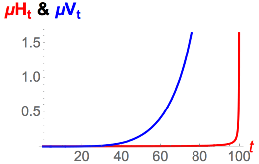
In both cases, there will be a vertical asymptote at $t=\omega$ . But how do the graphs compare? I made static graphs and put them in the same picture below. For Model $H$ , I chose $p=0.2$ . And for Model $V$ , I chose $p=5$ . Once again, at least for the values of $p$ chosen, model $V$ (blue) seems more realistic. It is less “extreme” in its behavior.

Forces of mortality. The red graph is Model $H$ , $\mu_{t}=\frac{p}{\omega-t}$ when $\omega=100$ and $p=0.2$ . The blue graph is Model $V$ , $\mu_{t}=\frac{pt^{p-1}}{\omega^{p}-t^{p}}$ when $\omega=100$ and $p=5$ . Once again, at least for the values of $p$ chosen, model $V$ (blue) seems more realistic. It is less ‘extreme’ in its behavior.

Probability Density Functions

The PDF for Model $H$ is the opposite of the derivative of its survival function: $-\frac{d}{dt}\left(\left(1-\frac{t}{\omega}\right)^{p}\right)=-p\left(1-\frac{t}{\omega}\right)^{p-1}\cdot \left(-\frac{1}{\omega}\right)=\frac{p}{\omega}\left(1-\frac{t}{\omega}\right)^{p-1}$ .

Likewise, the PDF for Model $V$ is $-\frac{d}{dt}\left(1-\frac{t^{p}}{\omega^{p}}\right)=\frac{p}{\omega^{p}}t^{p-1}$ .

Static graphs of these in the same situations as above are shown below. Once again, Model $V$ (blue) seems to be more realistic (the red graph actually has a vertical asymptote at $t=\omega$ since $p-1=0.2-1=-0.8$ in that case).

Probability Density Functions. The red graph is Model $H, f_{0}(t)=\frac{p}{\omega}\left(1-\frac{t}{\omega}\right)^{p-1}$ when $\omega=100$ and $p=0.2$ . The blue graph is Model $V, f_{0}(t)=\frac{p}{\omega^{p}}t^{p-1}$ when $\omega=100$ and $p=5$ . Once again, at least for the values of $p$ chosen, model $V$ (blue) seems more realistic. It is less ‘extreme’ in its behavior.

Probability Density Functions. The red graph is Model $H, f_{0}(t)=\frac{p}{\omega}\left(1-\frac{t}{\omega}\right)^{p-1}$ when $\omega=100$ and $p=0.2$ . The blue graph is Model $V, f_{0}(t)=\frac{p}{\omega^{p}}t^{p-1}$ when $\omega=100$ and $p=5$ . Once again, at least for the values of $p$ chosen, model $V$ (blue) seems more realistic. It is less ‘extreme’ in its behavior.

General Survival Functions and Complete Expectations of Life

General Survival Functions

Assuming survival to age $x>0$ , the continuous remaining lifetime random variable is $T_{x}=T_{0}-x$ . The conditional survival function (SF) is $\,_{t}p_{x}=\frac{S_{0}(x+t)}{S_{0}(x)}$ , the conditional force of mortality (FM) is $\mu_{x+t}$ , and the conditional probability density function (PDF) is $f_{x}(t)=-\frac{d}{dt}\left(\,_{t}p_{x}\right)=\,_{t}p_{x}\mu_{x+t}$ .

I will leave it as an exercise for you to check the following formulas:

(Model H) The SF is $\,_{t}p_{x}=\left(\frac{\omega-x-t}{\omega-x}\right)^{p}=\left(1-\frac{t}{\omega-x}\right)^{p}$ , the FM is $\mu_{x+t}=\frac{p}{\omega-x-t},$ and the PDF is $f_{x}(t)=\frac{p}{\omega-x-t}\left(\frac{\omega-x-t}{\omega-x}\right)^{p}=\frac{p}{(\omega-x)^{p}}\left(1-\frac{t}{\omega-x}\right)^{p-1}$ .
(Model V) The SF is $\,_{t}p_{x}=\frac{\omega^{p}-(x+t)^{p}}{\omega^{p}-x^{p}}$ , the FM is $\mu_{x+t}=\frac{p(x+t)^{p-1}}{\omega^{p}-(x+t)^{p}},$ and the PDF is $f_{x}(t)=\frac{p}{\omega^{p}-x^{p}}(x+t)^{p-1}$ .

Complete Expectation of Life

The complete expectation of life is the mean (expected value) of $T_{x}$ . It is denoted by $\stackrel{\circ}e_{x}$ and is defined by $\stackrel{\circ}e_{x}=E[T_{x}]=\displaystyle\int_{0}^{\infty}tf_{x}(t)dt=\displaystyle\int_{0}^{\infty}\,_{t}p_{x}dt$ .

For Model $H$ , the relevant integral to do is $\stackrel{\circ}e_{x}=\displaystyle\int_{0}^{\omega-x}\left(1-\frac{t}{\omega-x}\right)^{p}\, dt$ . This can be done with a substitution: $u=1-\frac{t}{\omega-x}$ so that $du=-\frac{1}{\omega-x}\, dt$ and $dt=-(\omega-x)\, du$ . After changing limits of integration and swapping them around to get rid of the minus sign, this gives $\stackrel{\circ}e_{x}=(\omega-x)\displaystyle\int_{0}^{1}u^{p}\, du=\frac{\omega-x}{p+1}$ .

For Model $V$ , the relevant integral to do is $\stackrel{\circ}e_{x}=\displaystyle\int_{0}^{\omega-x}\frac{\omega^{p}-(x+t)^{p}}{\omega^{p}-x^{p}}\, dt$ . This can be rewritten as $\frac{\omega^{p}(\omega-x)}{\omega^{p}-x^{p}}-\frac{1}{\omega^{p}-x^{p}}\displaystyle\int_{0}^{\omega-x}(x+t)^{p}\, dt$ . The last integral is $\displaystyle\int_{0}^{\omega-x}(x+t)^{p}\, dt=\frac{(x+t)^{p+1}}{p+1}\biggr\rvert_{t=0}^{t=\omega-x}=\frac{\omega^{p+1}-x^{p+1}}{p+1}$ .

Therefore, for Model $V$ , we have $\stackrel{\circ}e_{x}=\frac{(p+1)\omega^{p}(\omega-x)+x^{p+1}-\omega^{p+1}}{(p+1)(\omega^{p}-x^{p})}$ .

So, while Model $V$ seemed to be more realistic than Model $H$ , we see that the formula for its conditional mean is much more complicated. Is this trade-off worth it? It probably is as long as you have the necessary computing technology.

Graphs of Complete Expectations of Life

How do the graphs of $\stackrel{\circ}e_{x}$ in these two situations compare? They are shown below. For Model $H$ , we use $p=0.2$ . And for Model $V$ , we use $p=5$ . I would say it’s difficult to say which complete expectation of life is more realistic here, though the blue one has more “complexity” to it since it is nonlinear.

The complete expectation of life functions. Model $H$ (with $\omega=100$ and $p=0.2$ ) is in red and is linear. Model $V$ (with $\omega=100$ and $p=5$ ) is in blue and is nonlinear. We have consistently been saying that Model $V$ seems more realistic for these choices of the parameters. This claim is not necessarily true just from looking at these graphs, though a linear $\stackrel{\circ}e_{x}$ might seem unrealistic just by the very fact that it is too simple.

Curtate Expectation of Life

Recall that the discrete curtate lifetime random variable is $K_{x}=\lfloor T_{x}\rfloor$ . Also recall that its probability mass function (PMF) is $P[K_{x}=k]=\,_{k}|q_{x}=\,_{k}p_{x}-\,_{k+1}p_{x}=\,_{k}p_{x}\cdot q_{x+k}$ . The mean of $K_{x}$ is the curtate expectation of life and is $e_{x}=\displaystyle\sum_{k=0}^{\infty}k\cdot \,_{k}|q_{x}=\displaystyle\sum_{k=1}^{\infty}\,_{k}p_{x}$ .

For Model $H$ , we have $\,_{k}p_{x}=\left(1-\frac{k}{\omega-x}\right)^{p}$ . Therefore, $e_{x}=\displaystyle\sum_{k=1}^{\lfloor\omega-x\rfloor}\left(1-\frac{k}{\omega-x}\right)^{p}$ .

For Model $V$ , we have $\,_{k}p_{x}=\frac{\omega^{p}-(x+k)^{p}}{\omega^{p}-x^{p}}$ . Therefore, $e_{x}=\displaystyle\sum_{k=1}^{\lfloor\omega-x\rfloor}\frac{\omega^{p}-(x+k)^{p}}{\omega^{p}-x^{p}}$ .

Neither of these sums is easy to simplify. We will therefore just be content to graph these functions of $x$ and compare them as we did for the complete expectations of life.

In fact, the end result is almost indistinguishable from the graph above.

The curtate expectation of life functions. Model $H$ (with $\omega=100$ and $p=0.2$ ) is in red. Model $V$ (with $\omega=100$ and $p=5$ ) is in blue. These graphs look almost indistinguishable from the ones above.

They are different functions, however. In fact, for Model $H$ , we can compute $\stackrel{\circ}e_{0}\approx 83.3$ and $e_{0}\approx 82.7$ . And for Model $V$ , we can compute $\stackrel{\circ}e_{0}\approx 83.3$ and $e_{0}\approx 82.8$ .

In both situations, we have $\stackrel{\circ}e_{x}\approx e_{x}+\frac{1}{2}$ , as emphasized in the previous article “Curtate Expectation of Life”.