
Studying for Exam LTAM, Part 1.5

An important principle in mathematical modeling is to start simple. For example, if you have a situation where a linear function matches the trend in your data, go ahead and use a linear function rather than, for example, a quadratic function.
If a simple model is not accurate enough, then you will want to use a more complicated model.
For example, a linear function is definitely not accurate enough as a representation of the distance fallen by an object under the influence of the Earth’s gravity. A quadratic function must be used in this situation.
So far in our discussions about continuous survival random variables (in this series on studying for actuarial exam LTAM), we have focused on two relatively simple models.
- Uniform Distribution (De Moivre’s Law): the probability density function (PDF) is piecewise constant (and constant over the time of life).
- Constant Force of Mortality (Exponential Distribution): the force of mortality is constant, resulting in a PDF and a survival function (SF) that are exponential decay functions.
In this post, we will discuss another simple model that has the potential to be somewhat more accurate for human lifetimes: triangular distributions (also see https://learnandteachstatistics.files.wordpress.com/2013/07/notes-on-triangle-distributions.pdf). These are continuous random variables whose PDFs have graphs that look like the triangle in the figure above. They have the potential to be somewhat accurate models of human lifetimes because they can model the following facts:
- Not many people die at very young or very old ages (where the values of the PDF are low).
- Most commonly, people die in the age-range of 50 to 90 years (where the values of the PDF are large — near the high “peak of the tent”).
One aspect of human mortality that such models do not account for is relatively high infant mortality. Very young humans (< 2 months old) are more susceptible to death than, for example, young humans between the ages of 1 and 10 years old.
Formula for the PDF in Terms of Two Parameters
Let 

")
")

We assume that there is some number 


In order to be a PDF, the area under this graph, which is the area of the triangle, must be equal to 1. If 


This means the slope of the first (left-most) piece of this graph is 
}.")
Therefore, over the interval ![[0,\omega],](https://s0.wp.com/latex.php?latex=%5B0%2C%5Comega%5D%2C&bg=ffffff&fg=000000&s=0 "[0,\omega],")
=\begin{cases}\frac{2}{\omega d}t & \mbox{if } 0\leq t\leq d \\ \frac{2}{\omega(d-\omega)}(t-\omega) & \mbox{if } d<t\leq \omega \end{cases}.")
In this formula, 

")
In the case of the graph at the top of this post, 

=\begin{cases}\frac{t}{4800} & \mbox{if } 0\leq t\leq 80 \\ -\frac{t-120}{2400} & \mbox{if } 80<t\leq 120\end{cases}")
Survival Function(s)
The survival function (SF) for ![S_{0}(t)=1-F_{0}(t)=P[T_{0}>t].](https://s0.wp.com/latex.php?latex=S_%7B0%7D%28t%29%3D1-F_%7B0%7D%28t%29%3DP%5BT_%7B0%7D%3Et%5D.&bg=ffffff&fg=000000&s=0 "S_{0}(t)=1-F_{0}(t)=P[T_{0}>t].")

=1-\frac{t^{2}}{\omega d}")
If 
=1-\left(\frac{d}{\omega}+\displaystyle\int_{d}^{t}\frac{2}{\omega(d-\omega)}(s-\omega)\, ds\right)")
After a bit of tricky algebra, when =\frac{(t-\omega)^{2}}{\omega(\omega-d)}")
Hence, =\begin{cases}1-\frac{t^{2}}{\omega d} & \mbox{if } 0\leq t\leq d \\ \frac{(t-\omega)^{2}}{\omega(\omega-d)} & \mbox{if } d<t\leq \omega\end{cases}")
When ")


=-f_{0}(t)")
 and .
and .Assuming survival to age 

In the case where 

}{S_{0}(x)}=\begin{cases}\frac{\omega d-(x+t)^{2}}{\omega d-x^{2}} & \mbox{if } 0\leq t\leq d-x \\ \frac{d(x+t-\omega)^{2}}{(\omega-d)(\omega d-x^{2})} & \mbox{if } d-x<t\leq \omega-x \end{cases}")
In the case where 
}{S_{0}(x)}=\left(\frac{x+t-\omega}{x-\omega}\right)^{2}")

The following animation shows the how the graph of 

Note that, for any fixed }")

}{S_{0}(x)}") as increases from 0 to 60, in the case where and .
as increases from 0 to 60, in the case where and .Force(s) of Mortality (Hazard Rate Function(s))
The force of mortality (FM) for a newborn is }{S_{0}(t)}")


The FM for an individual ")
}{\omega d-(x+t)^{2}} & \mbox{if } 0<t<d-x \\ \frac{2}{\omega-x-t} & \mbox{if } d-x<t<\omega-x \end{cases}")
The following animation shows the how the graph of 
Note that there is a vertical asymptote at 


}{S_{0}(x+t)}") as increases from 0 to 60, in the case where and .
as increases from 0 to 60, in the case where and .Complete Expectation of Life
The complete expectation of life is, for this example with limiting age
![\stackrel{\circ}e_{x}=E[T_{x}]=\displaystyle\int_{0}^{\omega-x}\,_{t}p_{x}\, dt.](https://s0.wp.com/latex.php?latex=%5Cstackrel%7B%5Ccirc%7De_%7Bx%7D%3DE%5BT_%7Bx%7D%5D%3D%5Cdisplaystyle%5Cint_%7B0%7D%5E%7B%5Comega-x%7D%5C%2C_%7Bt%7Dp_%7Bx%7D%5C%2C+dt.&bg=ffffff&fg=000000&s=0 "\stackrel{\circ}e_{x}=E[T_{x}]=\displaystyle\int_{0}^{\omega-x}\,_{t}p_{x}\, dt.")
When 


Below is a static graph of 
It turns out that this second function is always an increasing function of
 and when and . The graph of is always increasing, no matter what the situation is.
You should make sure you understand the real-life meaning of the complete expectation of life. In this model, it turns out that 
As another example, for a person who is currently age 80, the model predicts an expected remaining lifetime of 
You might also wonder whether anything special is happening for this graph at 
One final animation is worth doing. What happens to the graph of
From this animation, we see that the mean remaining lifetimes are getting larger as the mode ")
As a final challenge, you might want to see if you can determine how
 as increases from 60 to 100. Note that the graph gets higher and steeper. The mean remaining lifetimes are getting larger as the mode increases, but they go down at a faster rate.
Mathematica Code
Below, for your reference, are pictures of the Mathematica code for the three animations above.
 when and as increases from 0 to 60.
 when and as increases from 0 to 60.
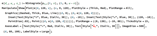 when increases from 60 to 100.