Measures of Spread in Survival Models - Infinity is Really Big

Studying for Exam LTAM, Part 1.6

One of the main lessons students should get out of any statistics course is the fact that quantitative data can be described with summary measures.

Data come with a wide variety of “locations”, “spreads”, and “shapes”. These words refer to the nature of the distribution of a given (random) variable quantity. The mean (arithmetic average) is the most common measure of “location”, or “central tendency”. The standard deviation is the most common measure of “spread”. Measures of “shape” can also be defined, but that is beyond the scope of this article.

For example, two basketball players can average the same number of points per game without being similar to each other, even when we only consider scoring points and ignore things like rebounding. One of the players could be very consistent in their scoring while the other could be very erratic. For the erratic player, very high scoring games would be offset by very low scoring games. The erratic player would have a higher standard deviation than the consistent player.

Likewise, the lengths of the lives of people from two different countries can have the same mean but different standard deviations. A larger standard deviation could occur, for example, in the country with a greater wealth disparity than the other.

The purpose of this article is to explore the way that standard deviations measure spread in three particular parametric survival models. The content to follow involves some calculations that are very intricate. This is especially true in the case of the third model we consider (a triangular distribution). If you are reading this for the first time, it is more important to understand the big picture. You should focus on understanding the meaning of the content. This is best done by thinking about the graphs. You can go back and check the calculations later.

Review: Measures of Location and Spread for Continuous Survival Random Variables

We have already discussed measures of location and spread of continuous survival random variables. This occurred in the article “Families of Continuous Survival Random Variables”. In this section, we briefly review that content.

In the sections after this, we will also consider how these ideas play out for specific models. The specific models (distributions) considered will be 1) uniform (De Moivre’s Law), 2) exponential, and 3) triangular.

Let $T_{0}$ be the age-at-failure for a newborn. Let $f_{0}(t)$ be the probability density function (PDF) of $T_{0}$ and $S_{0}(t)=P[T>t]$ be the survival function (SF) of $T_{0}$ . Assuming survival to age $x>0,$ we let $T_{x}=T_{0}-x$ be the remaining life random variable with conditional PDF $f_{x}(t)$ and conditional SF $\,_{t}p_{x}=S_{x}(t)=\frac{S_{0}(x+t)}{S_{0}(x)}=P[T_{x}>t|T_{0}>x]$ .

The mean is our fundamental measure of location (central tendency). Under reasonable assumptions about $\,_{t}p_{x}$ , the mean of $T_{x}$ is $\stackrel{\circ}e_{x}=E[T_{x}]=\displaystyle\int_{0}^{\infty}t f_{x}(t)\, dt=\displaystyle\int_{0}^{\infty}\,_{t}p_{x}\, dt$ . This is also called the complete expectation of life.

Under similar reasonable assumptions, the second moment of $T_{x}$ is $E[T_{x}^{2}]=\displaystyle\int_{0}^{\infty}t^{2}f_{x}(t)\, dt=\displaystyle\int_{0}^{\infty}2t \,_{t}p_{x}\, dt$ .

Our measures of spread are then the variance $\mbox{Var}(T_{x})=E[T_{x}^{2}]-\left(\stackrel{\circ}e_{x}\right)^{2}$ and the corresponding standard deviation $\sigma_{x}=\sqrt{\mbox{Var}(T_{x})}$ .

Our most basic (rough) interpretation of $\sigma_{x}$ in relation to $\stackrel{\circ}e_{x}$ is the following. For any distribution, almost all of the data/probability will be within 2 standard deviations of the mean.

Therefore, the more “spread out” the data/probabilities are, the larger the standard deviation. That is why it is a measure of “spread”.

Means for the Three Parametric Survival Models

We now summarize the results of these calculations for the means of the three parametric survival models mentioned above. You should take the time to check all these facts after your initial read-through of this article.

(Uniform Distribution — De Moivre’s Law) For $0\leq x<\omega$ , the conditional PDF is $f_{x}(t)=\frac{1}{\omega-x}$ for $0\leq t\leq \omega-x$ and the conditional SF is $\,_{t}p_{x}=1-\frac{t}{\omega-x}$ for $0\leq t\leq \omega-x$ . In this situation, the conditional mean is $\stackrel{\circ}e_{x}=\frac{\omega-x}{2}$ for $0\leq x<\omega$ . In other words, the expected remaining lifetime of someone age $x$ is half of the time left until they reach the maximum possible age $\omega$ . This makes sense because deaths are uniformly distributed over the interval.
(Exponential Distribution — Constant Force) For $\lambda>0$ , the conditional PDF is $f_{x}(t)=\lambda e^{-\lambda t}$ for $t\geq 0$ and the conditional SF is $\,_{t}p_{x}=e^{-\lambda t}$ for $t\geq 0$ . In this situation, the conditional mean is $\stackrel{\circ}e_{x}=\frac{1}{\lambda}$ for $x\geq 0$ . This is a constant function of $x$ — recall that this distribution is memoryless. It does not matter how old a person is, their expected remaining lifetime is unchanged. This is obviously not realistic over a long period of time.
(Triangular Distribution — read the article “Triangular Survival Models” first to help you understand this) In this situation, the formulas are far more complicated. They are also “piecewise-defined”. For $0\leq x< d<\omega$ and $0\leq t\leq \omega-x$ , we have $f_{x}(t)=\begin{cases}\frac{2(x+t)}{\omega d-x^{2}} & \mbox{if }0\leq t\leq d-x \\ \frac{2d(x+t-\omega}{(d-\omega)(\omega d-x^2)} & \mbox{if } d-x<t\leq \omega-x \end{cases}$ and $\,_{t}p_{x}=\frac{S_{0}(x+t)}{S_{0}(x)}=\begin{cases}\frac{\omega d-(x+t)^{2}}{\omega d-x^{2}} & \mbox{if } 0\leq t\leq d-x \\ \frac{d(x+t-\omega)^{2}}{(\omega-d)(\omega d-x^{2})} & \mbox{if } d-x<t\leq \omega-x \end{cases}$ . On the other hand, if $0<d\leq x<\omega$ , then $f_{x}(t)=-\frac{2(x+t-\omega)}{(\omega-x)^{2}}$ and $\,_{t}p_{x}=\frac{S_{0}(x+t)}{S_{0}(x)}=\left(\frac{x+t-\omega}{x-\omega}\right)^{2}$ for $0\leq t\leq \omega-x$ . When $d=80$ and $\omega=120$ , the graphs of $f_{0}(t)$ , $f_{40}(t)$ , $f_{100}(t)$ , $\,_{t}p_{0}$ $\,_{t}p_{40}$ , and $\,_{t}p_{100}$ are shown below. The conditional mean in this situation is described even further below.

The graph of the unconditional PDF $f_{0}(t)$ and the graphs of the conditional PDFs $f_{x}(t)$ when $x=40,100$ , for the triangular distribution with $d=80$ and $\omega=120$ .

The graph of the unconditional PDF $f_{0}(t)$ and the graphs of the conditional PDFs $f_{x}(t)$ when $x=40,100$ , for the triangular distribution with $d=80$ and $\omega=120$ .

*The graph of the unconditional SF $S_{0}(t)=\,_{t}p_{0}$ and the graphs of the conditional SFs $\,_{t}p_{x}$ when $x=40,100$ , for the triangular distribution with $d=80$ and $\omega=120$ .*

*The graph of the unconditional SF $S_{0}(t)=\,_{t}p_{0}$ and the graphs of the conditional SFs $\,_{t}p_{x}$ when $x=40,100$ , for the triangular distribution with $d=80$ and $\omega=120$ .*

In the triangular model (3) above, to find the conditional mean (complete expectation of life) $\stackrel{\circ}e_{x}$ , we again need to separate the problem into cases. If $0\leq x<d<\omega$ , then $\stackrel{\circ}e_{x}=\displaystyle\int_{0}^{d-x}\frac{\omega d-(x+t)^{2}}{\omega d-x^{2}}\, dt+\displaystyle\int_{d-x}^{\omega-x}\frac{d(x+t-\omega)^{2}}{(\omega-d)(\omega d-x^{2})}\, dt$ . If $0\leq d<x<\omega$ , then $\stackrel{\circ}e_{x}=\displaystyle\int_{0}^{\omega-x}\left(\frac{x+t-\omega}{x-\omega}\right)^{2}\, dt$ .

As an exercise, you should take the time to confirm that $\stackrel{\circ}e_{x}=\begin{cases}\frac{x^{3}-3x \omega d+\omega d^{2}+\omega^{2} d}{3\omega d-3x^{2}} & \mbox{if }0<x<d<\omega \\ \frac{\omega-x}{3} & \mbox{if } 0<d\leq x<\omega \end{cases}$ .

The graph of this function, along with the function $x+\stackrel{\circ}e_{x}$ , when $d=80$ and $\omega=120$ is shown below.

The reason that $x+\stackrel{\circ}e_{x}$ is shown is that it is always increasing, no matter what survival model is used. This should make sense. A person’s age plus their expected (mean) remaining lifetime should increase as they grow older.

Graphs of $\stackrel{\circ}e_{x}$ and $x+\stackrel{\circ}e_{x}$ when $d=80$ and $\omega=120$ for the triangular distribution. The graph of $x+\stackrel{\circ}e_{x}$ is always increasing, no matter what survival model is used.

Standard Deviations for the Three Parametric Survival Models

Now we summarize the results of the standard deviations for these models. As emphasized above, to help us complete this task, we must compute second moments and variances first. You should check all these calculations as well after your initial read-through.

Uniform Distribution (De Moivre’s Law)

For a uniform distribution the second moment is $E[T_{x}^{2}]=2\displaystyle\int_{0}^{\omega-x}t \,_{t}p_{x}\, dt=2\displaystyle\int_{0}^{\omega-x}\left(t-\frac{t^{2}}{\omega-x}\right)\, dt=\frac{(\omega-x)^{2}}{3}$ .

This leads to the variance $\mbox{Var}(T_{x})=\frac{(\omega-x)^{2}}{3}-\left(\frac{\omega-x}{2}\right)^{2}=\frac{(\omega-x)^{2}}{12}$ and standard deviation $\sigma_{x}=\sqrt{\mbox{Var}(T_{x})}=\frac{\omega-x}{\sqrt{12}}\approx 0.288675(\omega-x)$ .

Exponential Distribution (Constant Force)

For an exponential distribution, integration-by-parts can be used to see that the second moment is $E[T_{x}^{2}]=2\displaystyle\int_{0}^{\infty}t \,_{t}p_{x}\, dt=2\displaystyle\int_{0}^{\infty}te^{-\lambda t}\, dt=\frac{2}{\lambda^{2}}$ .

This leads to the variance $\mbox{Var}(T_{x})=\frac{2}{\lambda^{2}}-\left(\frac{1}{\lambda}\right)^{2}=\frac{1}{\lambda^{2}}$ and standard deviation $\sigma_{x}=\frac{1}{\lambda}$ . Once again, note that these quantities are constant in $x$ .

Triangular Distribution

Now you have your work cut out for you. If $0\leq x<d<\omega$ , you should check that the second moment is $E[T_{x}^{2}]=2\displaystyle\int_{0}^{\omega-x}t \,_{t}p_{x}\, dt=\frac{-x^{4}+\omega d^{3}-4x \omega d^{2}+6x^{2}\omega d+\omega^{2}d^{2}-4x\omega^{2}d+\omega^{3}d}{6(\omega d-x^{2})}.$ And if $0<d\leq x<\omega$ , the answer is the much simpler expression $E[T_{x}^{2}]=\frac{(\omega-x)^{2}}{6}$ .

For the variance, when $0\leq x<d<\omega$ , you should then get $\mbox{Var}(T_{x})=\frac{x^{6}-9x^{4}\omega d+8x^{3}\omega d(\omega+d)+\omega^{2}d^{2}(d^{2}-\omega d+\omega^{2})-3x^{2}\omega d(d^{2}+\omega d+\omega^{2})}{18(\omega d-x^{2})^{2}}$ . And if $0<d\leq x<\omega$ , we get $\mbox{Var}(T_{x})=\frac{(\omega-x)^{2}}{18}$ .

Of course, the standard deviations in these cases are the square roots of the variances. When $0\leq x<d<\omega$ , it is not even obvious that the variance is positive (though it must be). When $0<d\leq x<\omega$ , the standard deviation is $\sigma_{x}=\frac{\omega-x}{\sqrt{18}}\approx 0.235702(\omega-x)$ .

All these calculations emphasize that computer algebra systems (CAS), such as Mathematica, are good not just for simulation and graphing, but also for computation. Personally-speaking, I made sure to check all of these on Mathematica.

Graphical Perspectives

Formulas such as these are certainly important and good for computational purposes. But graphs are more helpful for understanding concepts and for seeing the big picture. For each of these three parametric survival models, it is helpful to make graphs of $\stackrel{\circ}e_{x}$ and $\stackrel{\circ}e_{x}\pm 2\sigma_{x}$ . This will serve to illustrate the visual interpretation of the standard deviation given in the review section near the beginning of this article and restated here. For any distribution, almost all of the data/probability will be within 2 standard deviations of the mean.

The animated graph below illustrates this visual interpretation for the uniform model $f_{x}(t)=\frac{1}{\omega-x}$ for $0\leq t\leq \omega-x$ . Again, in this situation, we have $\stackrel{\circ}e_{x}=\frac{\omega-x}{2}$ and $\sigma_{x}\approx 0.288675(\omega-x)$ so that $2\sigma_{x}\approx 0.577350(\omega-x)$ . In the animation, $\omega$ varies between 80 and 120 while $x$ varies between 0 and 60.

Note that for the graph on the left, “all the probability” (colored magenta) is between the two blue lines (within 2 standard deviations of the mean). This is true no matter what $\omega$ and $x$ are.

On the left, the graphs of $\stackrel{\circ}e_{x}$ and $\stackrel{\circ}e_{x}\pm 2\sigma_{x}$ are shown, along with a vertical line whose points have first coordinate equal to $x$ and whose second coordinates vary between 0 and $\omega-x$ . On the right, we see the PDF $f_{x}(t)=\frac{1}{\omega-x}$ for $0\leq t\leq \omega-x$ along with the locations of the points $\stackrel{\circ}e_{x}$ and $\stackrel{\circ}e_{x}\pm 2\sigma_{x}$ on the horizontal axis. Note that for both graphs, ‘all the probability’ is within 2 standard deviations of the mean, no matter what $\omega$ and $x$ are. In the animation, $\omega$ varies between 80 and 120 while $x$ varies between 0 and 60.

There’s not much point in making a similar animation for the exponential (constant force) model because nothing changes as $x$ changes (and there is no maximum age $\omega$ ). So we content ourselves with making a similar animation for the triangular distribution. It is shown below. Once again, notice that “almost all” of the probability is within 2 standard deviations of the mean.

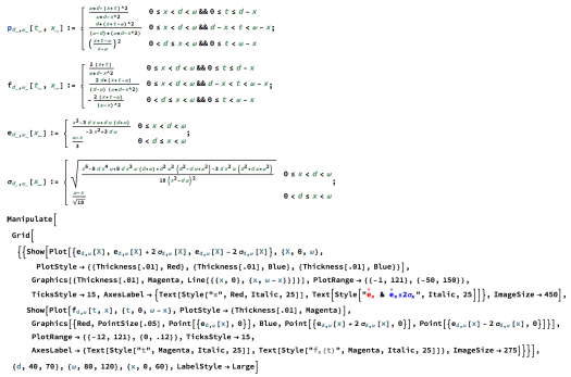
The Mathematica code to make these last two animations is shown in the screenshots below.