Visual Linear Algebra Online, Section 1.3

*Visualizing the parametric vector form of the solution set of a system with infinitely many solutions.*

Jack and Jill earn a combined $79.50 when Jack works 2 hours and Jill works 3 hours. On the other hand, if Jack works 3 hours and Jill works 2 hours, they make $78.75 total. What are their individual hourly pay rates?

This is a typical kind of problem you might encounter in a situation where there are two unknowns. In this case, the unknowns are Jack’s and Jill’s individual pay rates. One approach to solving this problem is to just make guesses.

In both situations, the total number of hours worked is five. In addition, the total amount of money earned in both situations is close to $79. Since $\frac{79\mbox{ dollars}}{5\mbox{ hours}}=15.80$ dollars per hour, we should expect both pay rates to be close to this amount.

Since the total amount earned is a bit more when Jill works more hours than Jack, we can say that Jill’s pay rate should be slightly higher than Jack’s pay rate. So, we might guess that Jack earns 15.50 $/hr and Jill earns 16.10 $/hr. This is probably not exactly right, but we can check how close it is as follows.

$2\mbox{ hrs}\times 15.50\frac{\$}{\mbox{hr}}+3\mbox{ hrs}\times 16.10\frac{\$}{\mbox{hr}}=\$31.00+\$48.30=\$79.30$ and

$3\mbox{ hrs}\times 15.50\frac{\$}{\mbox{hr}}+2\mbox{ hrs}\times 16.10\frac{\$}{\mbox{hr}}=\$46.50+\$32.20=\$78.70$ .

These are very close to the actual amounts $79.50 and $78.75 from above, so the correct answers for the pay rates would just take a bit more tweaking to find. However, we could easily end up guessing another five or six times before we come upon the exact right answers.

Use Algebra!

A better approach is to use algebra!

Represent their pay rates by letters which are “unknowns”. Suppose $x$ is Jack’s hourly pay rate, in dollars per hour, while $y$ is Jill’s hourly pay rate, in dollars per hour. If Jack works 2 hours, then his total pay is $2x$ dollars. If Jill works 3 hours, then her total pay is $3y$ dollars. Their total pay in this situation is $2x+3y$ , which must equal $79.50. Likewise, $3x+2y$ must equal $78.75. The resulting system of linear equations, shown without specifying the units, is below.

$\begin{cases}2x+3y=79.50 \\ 3x+2y=78.75\end{cases}$

We use the curly bracket symbol { to emphasize that these two equations are a “system”. They “go together”.

A system of equations like this is called an open sentence. This means it is neither true nor false. The open sentence only becomes true or false upon substitution of particular pair of numbers.

A solution of this system is a pair of numbers $(x,y)$ that makes the open sentence true. In other words, when you plug both numbers into both equations, you get a true statement.

In the present example, the unique solution is the pair $(x,y)=(15.45,16.20)$ . You can check this by substitution:

$2\mbox{ hrs}\times 15.45\frac{\$}{\mbox{hr}}+3\mbox{ hrs}\times 16.20\frac{\$}{\mbox{hr}}=\$30.90+\$48.60=\$79.50$ and

$3\mbox{ hrs}\times 15.45\frac{\$}{\mbox{hr}}+2\mbox{ hrs}\times 16.20\frac{\$}{\mbox{hr}}=\$46.35+\$32.40=\$78.75$ .

Of course, this begs a question. How did we find the unique solution?

There are two main methods: substitution and elimination.

Substitution

In the method of substitution, we use algebra techniques in the following order.

Solve one of the equations for one of the variables (it doesn’t matter which equation or which variable).
Substitute the answer from step 1 into the other equation in place of the variable that was solved for. That other equation will now only involve one variable, so solve for it.
Plug the answer from step 2 into any of the equations involving the two unknowns to solve for the other variable.

Substitution Details for Jack and Jill’s Pay Rates

Let us see how this works for the current system.

$\begin{cases}2x+3y=79.50 \\ 3x+2y=78.75\end{cases}$

In step 1, we will solve the first equation for $y$ . Here are the algebra steps.

$2x+3y=79.50\Longrightarrow 3y=79.50-2x\Longrightarrow y=\frac{79.5}{3}-\frac{2}{3}x=26.5-\frac{2}{3}x$ .

Now for step 2. In the second equation $3x+2y=78.75$ of the original system, substitute $26.5-\frac{2}{3}x$ in place of $y$ to get $3x+2(26.5-\frac{2}{3}x)=78.75$ . This can now be solved for $x$ . First, simplify to get $3x+53-\frac{4}{3}x=78.75$ and then $\frac{5}{3}x+53=78.75$ . The final algebra steps are below.

$\frac{5}{3}x+53=78.75\Longrightarrow \frac{5}{3}x=78.75-53=25.75$

$\Longrightarrow x=\frac{3}{5}\cdot 78.75-\frac{3}{5}\cdot 53=47.25-31.8=15.45$ .

This is the correct value for $x$ above, but we are not done. The unique solution must also involve the value of $y$ .

In step 3, we plug $x=15.45$ into the equation $y=26.5-\frac{2}{3}x$ to get the value of the other unknown $y=26.5-\frac{2}{3}\cdot 15.45=26.5-10.30=16.20$ .

The unique final answer is the ordered pair $(x,y)=(15.45,16.20)$ . This is one answer, not two separate answers.

Technically-speaking, checking that this solves the original system does more than just confirm that we are right. It actually proves we are right. All the algebra that we have done just confirms that this ordered pair is the only possible solution. It does not prove it is an actual solution.

We will discuss this more when we look at extraneous solutions (to nonlinear equations) further below.

Elimination

The second method is called the method of elimination. For this method, we attempt to rewrite the original system in equivalent forms so that one of the variables is “eliminated” (deleted) from each equation.

Once again, logically-speaking, this will only serve to derive possible solutions. The proof that we have derived true solutions is in the checking.

Start by observing the nature of the original system.

$\begin{cases}2x+3y=79.50 \\ 3x+2y=78.75\end{cases}$

If we multiply the top equation by 3 and the bottom equation by 2, there will be a $6x$ term in both equations. Because of this, we could then subtract the second equation from the first to obtain another equation not involving $x$ that must hold true for a solution pair $(x,y)$ . Here are the details:

$\begin{cases} 3\cdot (2x+3y)=3\cdot 79.50 \\ 2\cdot(3x+2y)=2\cdot 78.75,\end{cases}\mbox{ or}$

$\begin{cases}6x+9y=238.50 \\ 6x+4y=157.50.\end{cases}$

Subtracting the second equation from the first results in $(6x-6x)+(9y-4y)=238.50-157.50$ , or $5y=81.00$ .

Of course, this last equation now can be quickly solved for $y$ and then substituted into either equation in the original system to reach the final answer. However, we prefer to be more systematic here for the benefit of generalizing the method to higher-dimensional problems that have more equations and more unknowns.

The New System

So instead, we say we now have a “new system” where the $x$ has been “eliminated” in the second equation. Note that we choose to rewrite the first equation back in its original form (this is not absolutely necessary, but it is slightly more convenient).

$\begin{cases}\begin{array}{rcl} 2x+3y & = & 79.50 \\ 5y & = & 81.00\end{array}\end{cases}$

Now we notice that if we multiply the first equation by 5 and the second equation by 3, then we can subtract the second equation from the first to get a “new” first equation where we have “eliminated” $y$ .

Below you will find the details. In the final step we divide the first equation by 10 and the second equation by 5.

$\begin{cases}\begin{array}{rcl} 10x+15y & = & 397.50 \\ 15y & = & 243.00\end{array}\end{cases}$

$\begin{cases}\begin{array}{rcl} 10x\ \ \ \ \ \ & = & 154.50 \\ 5y & = & 81.00\end{array}\end{cases}$

and

$\begin{cases}\begin{array}{rcl} x\ \ \ \ \ \ & = & 15.45 \\ y & =& 16.20\end{array}\end{cases}$

We are purposely formatting the resulting systems in an odd way (with the $x$ terms further to the left) because that will help us relate these ideas to “row operations” with matrices later in Chapter 1.

Visualizing Systems and Their Solutions in Rectangular Coordinates

The facts that 1) linear equations have graphs which are straight lines in rectangular coordinates and 2) solutions of linear equations are ordered pairs $(x,y)$ are big hints that it should be helpful to visualize solutions in the rectangular coordinate plane.

We consider a new example.

$\begin{cases}\begin{array}{rcl} 5x-3y & = & 11 \\ x+2y & = & 10\end{array}\end{cases}$

Instead of fully solving this system right away using either substitution or elimination, let us graph both linear equations in the plane first, using rectangular coordinates.

Recall that the graph, in rectangular coordinates, of an equation in two unknowns $x$ and $y$ is the set of all points in the plane whose rectangular coordinates $(x,y)$ satisfy the equation.

To make these graphs, solve each equation for $y$ as a function of $x$ first, as discussed in Section 1.1, “Points, Coordinates, and Graphs in Two Dimensions”.

For the first equation $5x-3y=11 \Longrightarrow -3y=11-5x\Longrightarrow y=\frac{5}{3}x-\frac{11}{3}$ . For the second, $x+2y=10\Longrightarrow 2y=10-x\Longrightarrow y=-\frac{1}{2}x+5$ .

Now you can either plot points or use the slopes and intercepts of these lines to make the following graphs.

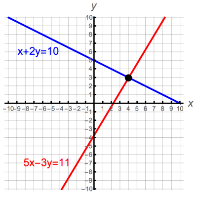
The graphs of the two equations in the linear system. Their point of intersection with rectangular coordinates $(x,y)=(4,3)$ is the unique solution of the system.

The graphs of the two equations in the linear system. Their point of intersection with rectangular coordinates $(x,y)=(4,3)$ is the unique solution of the system.

Since any solution $(x,y)$ to the system must satisfy both equations, any solution must lie on both lines. But these lines have only one point in common (their intersection consists of one point). This point appears to have rectangular coordinates $(x,y)=(4,3)$ .

We can easily check (prove!) that this is a solution to the system: $5\cdot 4-3\cdot 3=20-9=11$ and $4+2\cdot 3=4+6=10$ .

But is it the only solution? And how could we have found it algebraically? Use our methods from above.

Substitution

We have already solved both equations for $y$ in terms of $x$ , so step 1 of the substitution method is complete. Actually, since we did this for both equations, step 2 can be modified. We can just set the resulting expressions equal to each other.

In this case, since the first equation of the system became $y=\frac{5}{3}x-\frac{11}{3}$ and the second became $y=-\frac{1}{2}x+5$ , we can set $\frac{5}{3}x-\frac{11}{3}=-\frac{1}{2}x+5$ and solve for $x$ .

Here are the steps.

$\frac{5}{3}x-\frac{11}{3}=-\frac{1}{2}x+5\Longrightarrow \frac{5}{3}x+\frac{1}{2}x=5+\frac{11}{3}\Longrightarrow \frac{13}{6}x=\frac{26}{3}\Longrightarrow x=\frac{26}{3}\cdot \frac{6}{13}=4$ .

From this we then get $y=\frac{5}{3}\cdot 4-\frac{11}{3}=\frac{9}{3}=3$ . If we want extra confirmation, note that $y=-\frac{1}{2}\cdot 4+5=-2+5=3$ as well.

This work proves that $(x,y)=(4,3)$ is the only possible solution to the linear system. Since we already knew it was a solution from the checking above, we can say that $(x,y)=(4,3)$ is the unique solution to the linear system.

Elimination

For the elimination method, we start by swapping the order of the equations. This is not absolutely necessary, but it is a standard “row operation” and make our next operations a little bit easier.

$\begin{cases}\begin{array}{rcl} 5x-3y & = & 11 \\ x+2y & = & 10\end{array}\end{cases} \longrightarrow\ \ \ \begin{cases}\begin{array}{rcl} x+2y & = & 10 \\ 5x-3y & = & 11\end{array}\end{cases}$

Now multiply the first equation by 5, leave the second equation unchanged (multiply it by 1), and then subtract the first equation from the second to obtain a “new” second equation. Also, even though we multiplied the first equation by 5 before the subtraction, keep the first equation unchanged in the system.

$\begin{cases}\begin{array}{rcl} x+2y & = & 10 \\ 5x-3y & = & 11\end{array}\end{cases}\longrightarrow\ \ \ \begin{cases}\begin{array}{rcl}x+2y & = & 10 \\ -13y & = & -39\end{array}\end{cases}$

We note that this operation also could have been conceptualized as multiplying the first equation by $-5$ and adding it to the second equation. In fact, this is a more common way of conceptualizing the operation.

Now divide the new second equation by $-13$ (multiply it by $-\frac{1}{13}$ ) to get a new second equation. After that, multiply that new second equation by $-2$ and add it to the first equation to get a new first equation. Here is how to display these steps.

$\begin{cases}\begin{array}{rcl}x+2y & = & 10 \\ 13y & = & 39\end{array}\end{cases}\longrightarrow\ \ \begin{cases}\begin{array}{rcl}x+2y & = & 10 \\ y & = & 3\end{array}\end{cases}\longrightarrow\ \ \begin{cases}\begin{array}{rcl}x\ \ \ \ \ & = & 4 \\ y & = & 3\end{array}\end{cases}$

It is good to see that we got the same answer as before. When you are first learning these techniques, you might want to try both methods on at least a few problems as a way to double-check your answers.

Visualizing Elimination as a Transformation

There is an interesting way that the process of elimination can be visualized. In particular, we will visualize each “elimination step” as a “transformation”. Let us start with the step where $x$ is eliminated.

$\begin{cases}\begin{array}{rcl} x+2y & = & 10 \\ 5x-3y & = & 11\end{array}\end{cases}\longrightarrow\ \ \ \begin{cases}\begin{array}{rcl}x+2y & = & 10 \\ -13y & = & -39\end{array}\end{cases}$

We can think of this step as a combination of smaller steps. Multiply the first equation by $-5$ , then add the new first equation to the second equation to obtain a new second equation, then revert to keeping the first equation as it is.

Now, instead of multiplying the first equation by $-5$ , let us imagine multiplying it by an unspecified quantity $t$ . Doing this gives a new first equation of $tx+2ty=10t$ which we will then add to the second equation to get a new second equation. Doing this, and reverting back to the original form of the first equation can be shown as follows.

$\begin{cases}\begin{array}{rcl} x+2y & = & 10 \\ 5x-3y & = & 11\end{array}\end{cases}\longrightarrow\ \ \ \begin{cases}\begin{array}{rcl}x+2y & = & 10 \\ (5+t)x+(-3+2t)y & = & 11+10t\end{array}\end{cases}$

Note that in the second equation $x$ will be eliminated if $t=-5$ . Also note that in the second equation $y$ will be eliminated if $t=\frac{3}{2}$ (we won’t do this, but it is interesting to note that it can be done). Finally, note that the second equation is in its original form if $t=0$ .

When $t\not=0$ , the second equation represents a different line than the graph of $5x-3y=11$ . However, the solution (point of intersection) for the original system is the same. This is because we have algebra steps that are valid and therefore create an equivalent system.

Animation 1

We can visualize how the graph of $(5+t)x+(-3+2t)y = 11+10t$ changes as $t$ varies from 0 down to $-5$ . It is quite interesting to watch. It seems that $t$ induces a rotation of the original line $5x-3y=11$ to a new horizontal line $-13y=-39$ , which is equivalent to $y=3$ .

The graphs of $x+2y=10$ and $(5+t)x+(-3+2t)y=11+10t$ as $t$ decreases from 0 down to $-5$ . When $t=-5$ , the equation is $-13y=-39$ , or $y=3$ , whose graph is horizontal. As $t$ changes, the original line transforms to a new horizontal line via a rotation about the solution at $(x,y)=(4,3)$ .. This is equivalent to eliminating $x$ . The intersection point stays the same because these systems are all equivalent for all $t$ .

The graphs of $x+2y=10$ and $(5+t)x+(-3+2t)y=11+10t$ as $t$ decreases from 0 down to $-5$ . When $t=-5$ , the equation is $-13y=-39$ , or $y=3$ , whose graph is horizontal. As $t$ changes, the original line transforms to a new horizontal line via a rotation about the solution at $(x,y)=(4,3)$ .. This is equivalent to eliminating $x$ . The intersection point stays the same because these systems are all equivalent for all $t$ .

Animation 2

The step to eliminate $y$ from the first equation can be visualized in a similar way. Our “current” equivalent system is

$\begin{cases}\begin{array}{rcl}x+2y & = & 10 \\ y & = & 3.\end{array}\end{cases}$

Now multiply the second equation by an unspecified parameter $t$ to get $ty=3t$ , add the result to the first equation to get a new first equation, then leave the second equation as it was. This leads to the following system.

$\begin{cases}\begin{array}{rcl}x+(2+t)y & = & 10+3t \\ y & = & 3\end{array}\end{cases}$

We can see from this that $y$ will be eliminated from the first equation when $t=-2$ . So let us visualize the graphs of these equations as $t$ decreases from 0 down to $-2$ .

The graphs of $y=3$ and $x+(2+t)y=10+3t$ as $t$ decreases from 0 down to $-2$ . When $t=-2$ , the transformed equation is $x=4$ , whose graph is vertical. As $t$ changes, the original line transforms to a new vertical line via a rotation about the solution at $(x,y)=(4,3)$ .. This is equivalent to eliminating $y$ . The intersection point stays the same because these systems are all equivalent for all $t$ .

The graphs of $y=3$ and $x+(2+t)y=10+3t$ as $t$ decreases from 0 down to $-2$ . When $t=-2$ , the transformed equation is $x=4$ , whose graph is vertical. As $t$ changes, the original line transforms to a new vertical line via a rotation about the solution at $(x,y)=(4,3)$ .. This is equivalent to eliminating $y$ . The intersection point stays the same because these systems are all equivalent for all $t$ .

As we saw above, the final answer is $(x,y)=(4,3)$ , because our original system was transformed to the equivalent system

$\begin{cases}\begin{array}{rcl}x\ \ \ \ \ & = & 4 \\ y & = & 3.\end{array}\end{cases}$

Are These Rotations Occurring at a Constant Rate?

One nice thing about visuals like this is that they can spur us to ask and try to answer interesting questions.

For example, do the angles of rotation change at constant rates in these animations? It is a bit tough to tell in the second animation. In the first one, it seems that perhaps the angle is changing faster when the line is steep than when it is flat.

But, appearances can be deceiving. It would be best to do some calculations to confirm what is going on.

Dot Product and Angles

Recall from from Section 1.2, “Vectors in Two Dimensions” that the angle between two nonzero vectors ${\bf v}$ and ${\bf w}$ can be related to the dot product. This angle is $\arccos\left(\frac{{\bf v}\cdot {\bf w}}{||{\bf v}|| ||{\bf w}||}\right)=\cos^{-1}\left(\frac{{\bf v}\cdot {\bf w}}{||{\bf v}|| ||{\bf w}||}\right)$ . In this formula, ${\bf v}\cdot {\bf w}$ is the dot product of ${\bf v}$ and ${\bf w}$ , while $||{\bf v}||=\sqrt{{\bf v}\cdot {\bf v}}$ and $||{\bf w}||=\sqrt{{\bf w}\cdot {\bf w}}$ are the lengths of ${\bf v}$ and ${\bf w}$ , respectively.

Choosing Vectors Parallel to the Lines

Consider the second animation above. One vector that is parallel to the horizontal red line is ${\bf w}=\left(\begin{array}{c} -4 \\ 0 \end{array}\right)$ .

For any fixed $t$ , the equation of the blue line is $x+(2+t)y=10+3t$ . If we solve this for $y$ as a function of $x$ , we get $y=-\frac{1}{2+t}x+\frac{10+3t}{2+t}$ . Thus, the line has slope $-\frac{1}{2+t}$ .

We would like to find a vector that stays parallel to the blue line as $t$ changes. If we let ${\bf v}$ be a vector whose first (horizontal) component is, for example, $-4$ , then ${\bf v}$ will be parallel to the blue line if we choose the second (vertical) component to be $-\frac{1}{2+t}\cdot (-4)=\frac{4}{2+t}$ .

In other words, ${\bf v}=\left(\begin{array}{c} -4 \\ \frac{4}{2+t} \end{array}\right)$ is parallel to the blue line for any fixed $t$ .

If we place the vectors ${\bf v}$ and ${\bf w}$ to have their initial points both at $(x,y)=(4,3)$ , we get the following animation as $t$ decreases from 0 down to $-1.5$ .

The vectors ${\bf v}$ and ${\bf w}$ are parallel to the blue and red lines, respectively. We are interested in whether the angle $\theta$ changes at a constant rate as $t$ decreases or not.

The vectors ${\bf v}$ and ${\bf w}$ are parallel to the blue and red lines, respectively. We are interested in whether the angle $\theta$ changes at a constant rate as $t$ decreases or not.

Angle Calculation

The length of ${\bf w}$ is constant: $||{\bf w}||=4$ . The length of ${\bf v}$ is a function of $t$ : $||{\bf v}||=\sqrt{(-4)^{2}+\left(\frac{4}{2+t}\right)^{2}}=\sqrt{\frac{16(2+t)^{2}+16}{(2+t)^{2}}}=\frac{\sqrt{80+64t+16t^{2}}}{2+t}$ .

In this last calculation, note that $\sqrt{(2+t)^{2}}=|2+t|=2+t$ since $t>-2$ .

Finally, the dot product of ${\bf v}$ and ${\bf w}$ is ${\bf v}\cdot {\bf w}=16$ .

Therefore, as a function of $t$ , the angle between the two lines is $\theta=\arccos\left(\frac{16}{4\cdot \frac{\sqrt{80+64t+16t^{2}}}{2+t}}\right)=\arccos\left(\frac{8+4t}{\sqrt{80+64t+16t^{2}}}\right)$ .

This is certainly not a linear function of $t$ . The angle $\theta$ definitely does not change at a constant rate in the second animation.

The graph of this function is shown below. Note that the derivative $\frac{d\theta}{dt}$ is everywhere negative, because the angle $\theta$ increases as the parameter $t$ decreases. Also note that the slope is steeper when $t$ is near $-1.5$ . In the animation, this means that the rotation starts slow and speeds up as $t$ decreases.

The angle $\theta$ as a function of the parameter $t$ . This graph is not a straight line. The rotation is **not** at a constant rate.

Classification of Two-Dimensional Linear Systems

What can we say about the general two-dimensional linear system?

$\begin{cases}\begin{array}{rcl} ax+by & = & u \\ cx+dy & = & v\end{array}\end{cases}$

Geometric Approach

Start by thinking geometrically (in rectangular coordinates). Assuming either $a\not=0$ or $b\not=0$ (or both), then the graph of $ax+by=u$ will be a straight line in the plane. Likewise, assuming either $c\not=0$ or $d\not=0$ (or both), then the graph of $cx+dy=v$ will also be a straight line in the plane.

Typically (“generically”), these two lines will have two different slopes. In that case, they will intersect at just one point, which will evidently be the unique solution of the linear system.

If the lines happen to have the same slope, then they will be parallel. If these two parallel lines are distinct, the lines will not intersect and the linear system will have no solution.

On the other hand, if these two parallel lines are actually the same parallel line, there will evidently be infinitely many solutions to the linear system (all the points on this common line).

Systems which have a solution are called consistent. Systems which do not have a solution are called inconsistent.

Algebraic Approach

How would this play out if we attempted to do row operations in the general case?

$\begin{cases}\begin{array}{rcl} ax+by & = & u \\ cx+dy & = & v\end{array}\end{cases}$

Unique Solutions

To keep things simple, assume that $a\not=0$ . To eliminate the $cx$ term from the second equation, multiply the first equation by $-\frac{c}{a}$ (with $a\not=0$ ). Then add this to the second equation, obtaining a new second equation (and reverting back to the original first equation). Below is the schematic representation of this operation, along with a second operation which is a multiplication of the second equation by $\frac{a}{ad-bc}$ .

$\begin{cases}\begin{array}{rcl} ax+by & = & u \\ cx+dy & = & v\end{array}\end{cases}\longrightarrow \begin{cases}\begin{array}{rcl} ax+by & = & u \\ \frac{ad-bc}{a}y & = & \frac{av-cu}{a}\end{array}\end{cases}\longrightarrow \begin{cases}\begin{array}{rcl} ax+by & = & u \\ y & = & \frac{av-cu}{ad-bc}\end{array}\end{cases}$

It is of utmost importance to note that the second operation above can only be performed if we also assume that $ad-bc\not=0$ . This is actually the condition that guarantees that the two original lines are not parallel, so there will be a unique solution.

The quantity $ad-bc$ is so important that it has a name. It is called the determinant of the linear system (more precisely, it is the determinant of the so-called coefficient matrix of the linear system).

Back-substitution of $y=\frac{av-cu}{ad-bc}$ in place of $y$ in the first equation of the system can now allow you to solve for $x$ (assuming $a\not=0$ ). The simplified answer is $x=\frac{du-bv}{ad-bc}$ .

Therefore, when $a\not=0$ and $ad-bc\not=0$ , the unique solution of the linear system is the ordered pair $\left(\frac{du-bv}{ad-bc},\frac{av-cu}{ad-bc}\right)$ .

It is an exercise to show that the same answer can be obtained when $a=0$ as long as $ad-bc\not=0$ .

Infinitely Many Solutions or No Solutions

On the other hand, if the determinant $ad-bc=0$ , the original system will either have no solutions or infinitely many solutions.

It is an exercise to show that there are infinitely many solutions if the equations $ax+by=u$ and $cx+dy=v$ are constant (nonzero) multiples of each other. In other words, when there is a nonzero constant $\lambda$ so that $c=\lambda a$ , $d=\lambda b$ , and $v=\lambda u$ . Note that it is possible that either $a=c=0$ or that $b=d=0$ in this situation.

It is also an exercise to show that there are no solutions when $ad-bc=0$ if there is a nonzero constant $\lambda$ such that $c=\lambda a$ and $d=\lambda b$ , but $v\not=\lambda u$ .

Parametric Vector Form of Solutions in the Infinite Case

Consider the case where $c=\lambda a$ , $d=\lambda b$ , and $v=\lambda u$ for $\lambda\not=0$ . In this case, the equations in the system are nonzero multiples of each other and there are infinitely many solutions.

Doing row operations in this situation will result in a second equation that is converted to $0=0$ . This means the second equation can be “discarded” or “ignored” and we can just focus on the first equation $ax+by=u$ .

In the case where $b\not=0$ , we can solve this for $y$ as a function of $x$ to get $y=-\frac{a}{b}x+\frac{u}{b}$ (and in the case where $b=0$ but $a\not=0$ , we can solve for $x$ as a function of $y$ ).

In this setting, it is customary to call $x$ a “free variable” and to write the infinitely many solutions in “parametric vector form” as shown below.

${\bf u}=\left(\begin{array}{c} x \\ y \end{array}\right)=\left(\begin{array}{c} x \\ -\frac{a}{b}x+\frac{u}{b} \end{array}\right)=\left(\begin{array}{c} 0 \\ \frac{u}{b} \end{array}\right)+x\left(\begin{array}{c} 1 \\ -\frac{a}{b}\end{array}\right)={\bf v}+x{\bf w}$

In doing this, we are: 1) viewing the solutions as vectors rather than as points (using the natural association between points and vectors discussed in Section 1.2, “Vectors in Two Dimensions”) and 2) treating the vectors ${\bf v}$ and ${\bf w}$ as “constant parts” of the solution, while allowing the real number $x$ to be the “variable part” (i.e., the “parameter”).

Because there is one (linear) parameter, the solution set can be at most one-dimensional. In fact, it is exactly one-dimensional and is, of course, a straight line.

Viewing Solutions in Terms of the Geometry of Vector Operations

If we place the initial point of ${\bf v}=\left(\begin{array}{c} 0 \\ \frac{u}{b} \end{array}\right)$ at the origin and the initial point of ${\bf w}=\left(\begin{array}{c} 1 \\ -\frac{a}{b}\end{array}\right)$ at the tip of ${\bf v}$ , then we can use the geometric interpretation of scalar multiplication and vector addition to view the infinitely many solution points in terms of these vectors.

For example, suppose the system is the following.

$\begin{cases}\begin{array}{rcl} 2x-y & = & 5 \\ -4x+2y & = & -10\end{array}\end{cases}$

These equations are constant multiples of each other and row operations will produce a second equation that can be discarded. The solution set is the line represented by $2x-y=5$ , which is equivalent to $y=2x-5$ . In parametric vector form, the solution set is represented in the following way.

${\bf u}={\bf v}+x{\bf w}=\left(\begin{array}{c} 0 \\ -5 \end{array}\right)+x\left(\begin{array}{c} 1 \\ 2 \end{array}\right)$

And here is a way to visualize the solution set that takes advantage of our understanding of the geometry of vector addition and scalar multiplication. As a set of points, the solution set is the green line. As a set of vectors, the solution set consists of all the magenta-colored (pink) vectors.

Visualizing the parametric vector form of the solution set of a system with infinitely many solutions. As a set of points, the solution set is the green line. As a set of vectors, the solution set consists of all the magenta-colored (pink) vectors.

Important Observations

Note that ${\bf v}=\left(\begin{array}{c} 0 \\ -5 \end{array}\right)$ is one particular solution to the original system.

$\begin{cases}\begin{array}{rcl} 2x-y & = & 5 \\ -4x+2y & = & -10\end{array}\end{cases}$

On the other hand, the vector ${\bf w}=\left(\begin{array}{c} 1 \\ 2 \end{array}\right)$ does not solve the original system. Instead, it solves the so-called corresponding homogeneous system, where the constants on the right-hand sides are both zero.

$\begin{cases}\begin{array}{rcl} 2x-y & = & 0 \\ -4x+2y & = & 0\end{array}\end{cases}$

This is an observation that will generalize to higher dimensions. Make sure you remember it for the future.

Relationship to Coordinate Changes

Consider once again the general linear system, written in a slightly different way.

$\begin{cases}\begin{array}{rcl} u & = & ax+by \\ v & = & cx+dy\end{array}\end{cases}$

As discussed in Section 1.1, “Points, Coordinates, and Graphs in Two Dimensions”, it will be helpful in future sections to think of these equations as defining a “linear transformation”. This linear transformation will essentially take a system of rectangular coordinates $(x,y)$ and convert it to a system of new coordinates $(u,v)$ for points in the plane. Most likely (generically), these new coordinates will be with respect to a system of slanted axes.

Assuming that the determinant $ad-bc\not=0$ , this linear transformation will have an inverse. Finding this inverse involves doing the exact same algebra as in the previous section where we found the unique solution $\left(\frac{du-bv}{ad-bc},\frac{av-cu}{ad-bc}\right)$ .

As a system of equations, the inverse transformation can be written as follows.

$\begin{cases}\begin{array}{rcl} x & = & \frac{d}{ad-bc}u-\frac{b}{ad-bc}v \\ y & = & -\frac{c}{ad-bc}u+\frac{a}{ad-bc}v\end{array}\end{cases}$

Extraneous Solutions of Nonlinear Equations

Finally, we re-emphasize the logical importance of checking solutions. Logically-speaking, the substitution or elimination steps to solve a system only derive possible solutions. The proof that we have found actual solutions is in the checking.

This point is brought home by considering certain nonlinear equations.

For example, consider the nonlinear equation $x-4=\sqrt{x+2}$ . To solve for $x$ , a standard first step is to square both sides to get rid of the radical. Doing so gives $(x-4)^{2}=x+2$ , which becomes $x^{2}-8x+16=x+2$ and then $x^{2}-9x+14=0$ . This quadratic can be factored to get $(x-2)(x-7)=0$ and get possible solutions of $x=2$ and $x=7$ .

However, if you check these in the original equation, only $x=7$ works. The number $x=2$ is not a solution of the original equation, since $\sqrt{2+2}=\sqrt{4}=2\not=-2=2-4$ (by definition, the symbol $\sqrt{4}$ only represents the positive square root of 4). We therefore call $x=2$ an extraneous solution of the original equation (a better term is probably “fictitious solution”).

The root of the problem here (pun intended) is that we squared both sides of the original equation $x-4=\sqrt{x+2}$ . Such a transformation is not invertible because it is not one-to-one.

Exercises

Bobby and Cindy earn a combined $134.70 when Bobby works 3 hours and Cindy works 4 hours. On the other hand, if Bobby works 4 hours and Cindy works 3 hours, they make $134.10 total. What are their individual hourly pay rates?
(a) Use both substitution and elimination to find the unique solution of the following system. Show your work. (b) Draw graphs in the plane (in rectangular coordinates) to represent this situation.

$\begin{cases}\begin{array}{rcl} 7x+5y & = & 11 \\ -3x+4y & = & 26 \end{array}\end{cases}$

3. (a) Represent the solutions of the following system in parametric vector form with $y$ as a free variable (rather than $x$ ). (b) Draw a picture of the line along with the vectors ${\bf u}$ , ${\bf v}$ , and ${\bf w}$ when $y=1$ .

$\begin{cases}\begin{array}{rcl} x+2y & = & 4 \\ 3x+6y & = & 12 \end{array}\end{cases}$

4. Verify that the solution of the general system below is $\left(\frac{du-bv}{ad-bc},\frac{av-cu}{ad-bc}\right)$ even in the case where $a=0$ as long as $ad-bc\not=0$ . Note that, in this case this also means you can assume $bc\not=0$ .

$\begin{cases}\begin{array}{rcl} ax+by & = & u \\ cx + dy & = & v \end{array}\end{cases}$

5. Show work to find the inverse transformation of the one defined by the following system. Assume you are never dividing by zero as you work through your steps.

$\begin{cases}\begin{array}{rcl} u & = & ax+by \\ v & = & cx+dy \end{array}\end{cases}$

Video for Section 1.3

Here is a video overview of the content of this section.

Systems of Linear Equations in Two Dimensions

Visual Linear Algebra Online, Section 1.3

Jack and Jill earn a combined $79.50 when Jack works 2 hours and Jill works 3 hours. On the other hand, if Jack works 3 hours and Jill works 2 hours, they make $78.75 total. What are their individual hourly pay rates?

Use Algebra!

Substitution

Substitution Details for Jack and Jill’s Pay Rates

Elimination

The New System

Visualizing Systems and Their Solutions in Rectangular Coordinates

Substitution

Elimination

Visualizing Elimination as a Transformation

Animation 1

Animation 2

Are These Rotations Occurring at a Constant Rate?

Dot Product and Angles

Choosing Vectors Parallel to the Lines

Angle Calculation

Classification of Two-Dimensional Linear Systems

Geometric Approach

Algebraic Approach

Unique Solutions

Infinitely Many Solutions or No Solutions

Parametric Vector Form of Solutions in the Infinite Case

Viewing Solutions in Terms of the Geometry of Vector Operations

Important Observations

Relationship to Coordinate Changes

Extraneous Solutions of Nonlinear Equations

Exercises

Video for Section 1.3

Next: Section 1.4, Linear Transformations in Two Dimensions